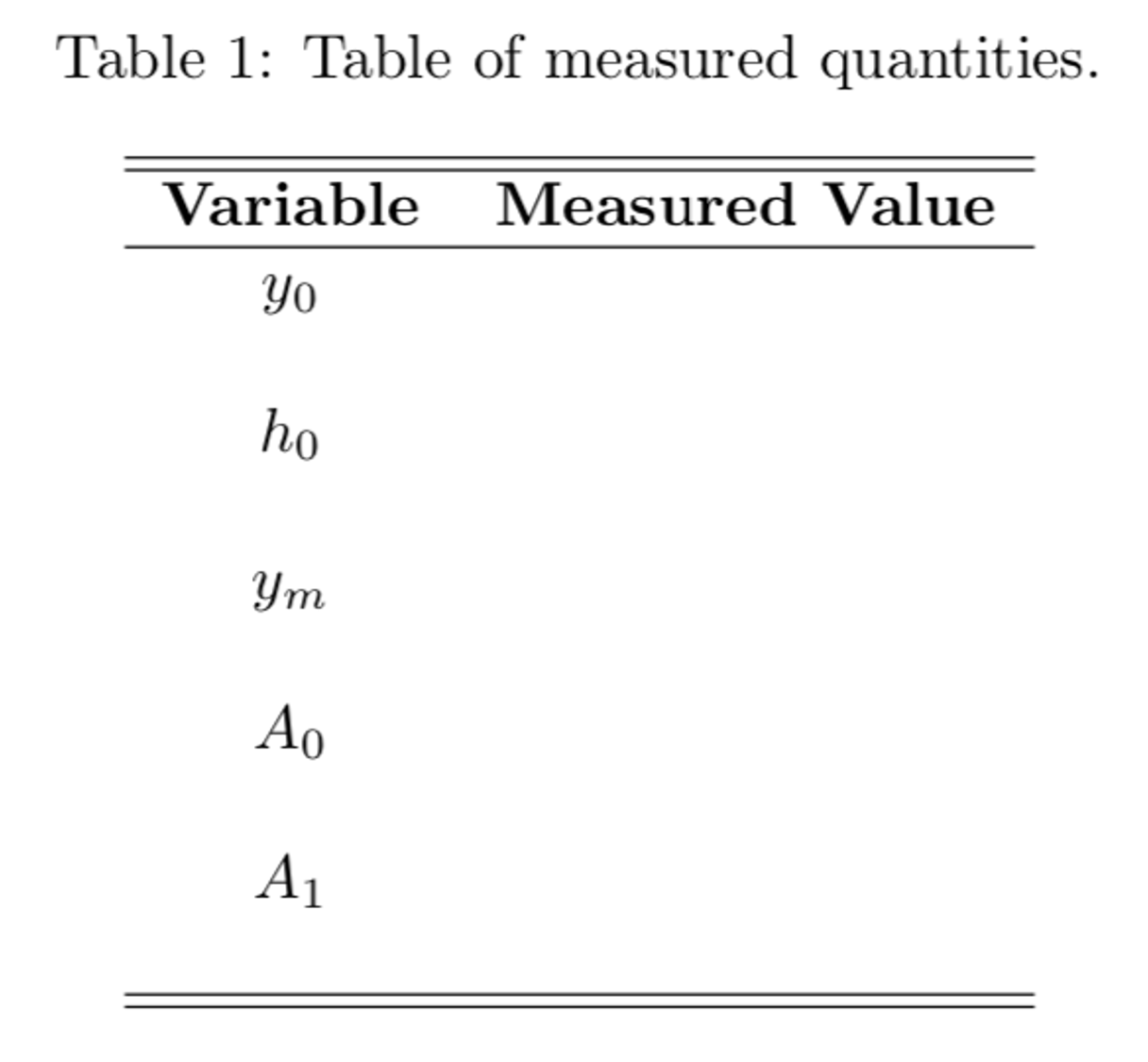
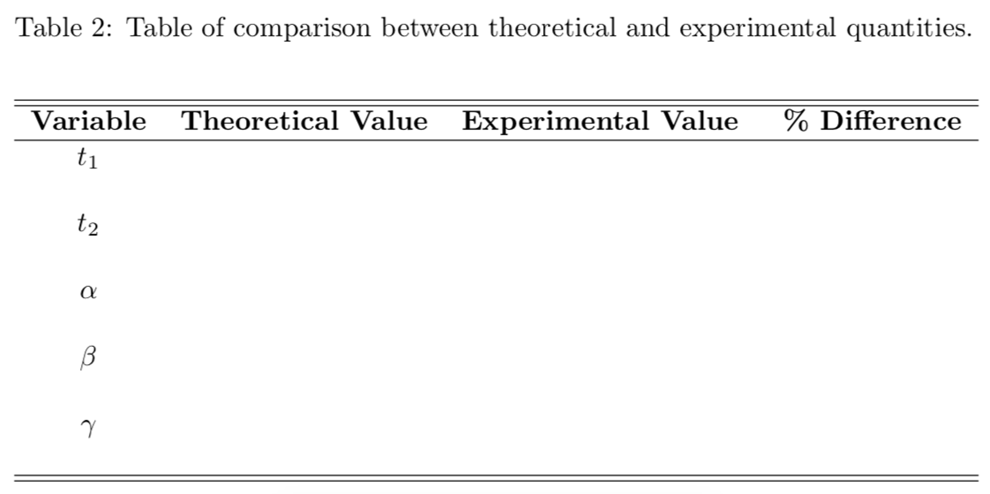
Physics Overview
Bernoulli's Principle along with the Equation of Continuity are the two central concepts to understand for describing laminar and inviscid flow. The former conveys the conservation of mechanical energy in fluid flow, while the latter conveys conservation of mass.
Consider the following experimental scenario: a mass \(m\) suspended in a can of water with the aid of a string as shown in Fig. 1. The volume of the mass is \(V\) and it has a uniform density \(\rho_0\), and we will assume it has a uniform cross-sectional area \(A_0\) and height \(h_0\), as shown. The tension in the string is \(T\). The can has a cylindrical cross-section of area \(A_1\) and it has a small orifice at the bottom, of cross-sectional area \(A_2\). Water streams out through the bottom orifice and the instantaneous velocity of the flow at the two cross-sections are \(v_1\) and \(v_2\) respectively.
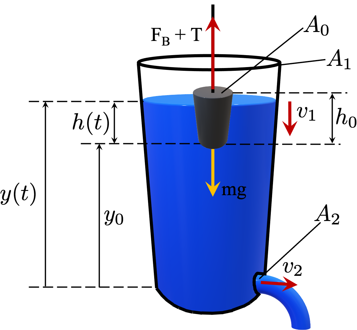
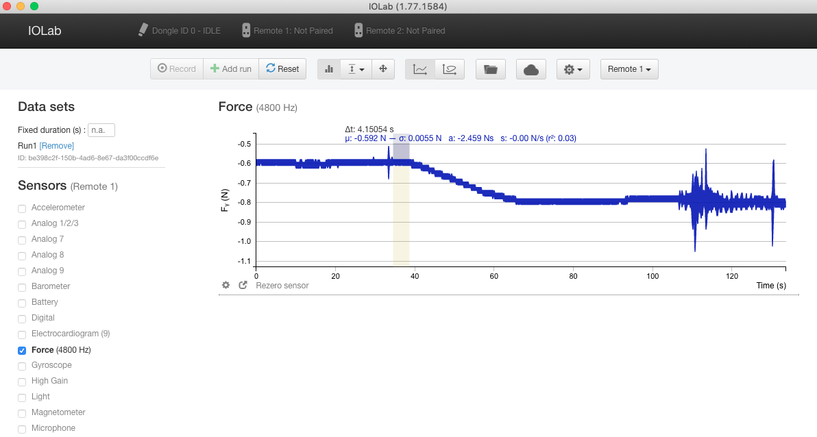
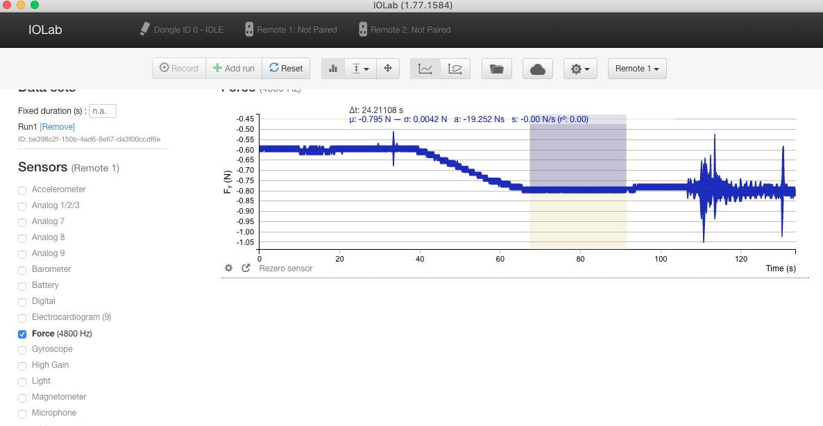
The height of the top surface of the water-level is \(y(t)\), measured from the bottom of the can. The orifice is located at \(y=0\). The small mass is initially fully submerged and then as the water level gradually drops it will become partially submerged at some point, and then some time later, the water-level will drop below the suspended mass. Suppose that at some arbitrary time \(t\), the amount of the small mass submerged is \(h(t)\). When \(y(t) \geq y_0 + h_0\) then \(T=mg-F_B\) and when \(y(t)\leq y_0\) then \(T=mg\). In between the tension will vary as a function of time. We will derive this precise relationship, and we will disover that it varies quadratically as a function of time, between an upper bound of \(mg\) and a lower bound of \(mg-F_B\).
Let us however start by examining the flow of the water. We will assume that the flow is laminar. We can apply the equation of continuity as well as Bernoulli's Equation to cross-sections \(1\) and \(2\) and write:
\[A v_1 = A_2 v_2\label{eq:eq_cont}\] and
\[ \underbrace{\frac{1}{2}\rho v_1^2 + \rho g y(t) + P_0}_{\textrm{at cross-section~}1} = \underbrace{\frac{1}{2}\rho v_2^2 + 0 + P_0}_{\textrm{at cross-section~}2} \label{eq:bernoulli_eq}\].
Where \(\rho\) is the density of water and \(A\) is the cross-sectional area of the top surface of the water level at some arbitrary time. Note that when the water-level \(y(t) > y_0 + h_0\) then the cross-sectional area at the top surface of the water-level is \(A_1\), however, when the water-level drops below the top-most part of the small mass, then cross-sectional area at the top surface of the water-level becomes \(A_1-A_0\). Then again when \(y(t) < y_0 \) the cross-sectional area again becomes equal to \(A_1\). It is only when the small mass is partly submerged that the cross-sectional area is reduced. We can therefore write:
\[ \begin{align} A = \left\{ \begin{array}{cc} A_1 & \hspace{5mm} y(t) > y_0 + h_0 \\ A_1 - A_0 & \hspace{5mm} y_0 \leq y(t) \leq y_0 + h_0 \\ A_1 & \hspace{5mm} y(t) < y_0 \\ \end{array} \right. \end{align}\]
Substituting Eq. \eqref{eq:eq_cont} into Eq. \eqref{eq:bernoulli_eq} we get after some algebra:
\[\left(\frac{A^2}{A_2^2}-1 \right)v_1^2 = 2g y(t), \] which yields
\[ \implies v_1 = \sqrt{\frac{2gy(t)}{A^2/A_2^2-1}}~.\]
Recognizing that
\[v_1 = -\frac{dy(t)}{dt},\] we get:
\[ \frac{dy}{dt} = -\sqrt{\frac{2gy}{A^2/A_2^2-1}}~.\label{eq:dydt}\]
Where we have written \(y \equiv y(t)\) for brevity.
Putting
\[ \kappa = \sqrt{\frac{2g}{A^2/A_2^2-1}},\] we get:
\[ \frac{dy}{dt} = -\kappa y^{1/2}~. \label{eq:ode}\]
This is an ordinary differential equation and can be integrated with ease, however care must be taken when performing the integral as the prefactor \(\kappa\) depends on the height of the water level.
\[ \begin{align} \kappa = \left\{ \begin{array}{cc} \kappa_1 & \hspace{5mm} y(t) > y_0 + h_0 \\ \kappa_2 & \hspace{5mm} y_0 \leq y(t) \leq y_0 + h_0 \\ \kappa_1 & \hspace{5mm} y(t) < y_0 \\ \end{array} \right. \end{align}\] where:
\[\kappa_1 = \sqrt{\frac{2g}{A_1^2/A_2^2-1}}\] and
\[\kappa_2 = \sqrt{\frac{2g}{(A_1-A_0)^2/A_2^2-1}}.\]
Suppose the initial level of the water is \(y_m\) at \(t=0\). Then we can integrate this differential equation in Eq. \eqref{eq:ode} in three parts depending on the prefactor \(\kappa\). First we integrate from the initial water-level (\(y_m\)) to some arbitrary time before the water-level drops to \(y_0+h_0\). For the second part of the integral we will then integrate from when the water-level drops from \(y_0+h_0\) to some some arbitrary level \(y>y_0\), and finally we will integrate from when the water-level drops from \(y_0\) to some arbitrary height \(y < y_0 \). Thus, we will obtain three different expressions for \(y(t)\). We have to do the same integral three times, in the three different regimes.
First let us look at the regime \(y_0+h_0 < y(t) < y_m \):
\[ \int_{y_m}^y\frac{dy}{\sqrt{y}} = -\int_0^t \kappa_1 dt, \] which immediately yields,
\[ 2\left(\sqrt{y}-\sqrt{y_m}\right) = - \kappa_1 t \]
\[ \implies y(t) = \left(\sqrt{y_m} - \frac{1}{2}\kappa_1 t\right)^2; \qquad y_0+h_0 < y(t) < y_m \label{eq:first_regime}\]
The time it takes for the water-level to drop from \(y_m\) to \(y_0+h_0\) is:
\[ t_1 = \frac{2\left(\sqrt{y_m} - \sqrt{y_0+h_0}\right)}{\kappa_1} \label{eq:t1}\]
Next, let us look at the second regime; \(y_0 < y(t) < y_0+h_0 \):
\[ \int_{y}^{y_0+h_0}\frac{dy}{\sqrt{y}} = -\int_{t_1}^t \kappa_2 dt, \] which immediately yields,
\[ 2\left(\sqrt{y_0+h_0}-\sqrt{y}\right) = - \kappa_2 (t-t_1) \]
\[ y(t) = \left(\sqrt{y_0+h_0} - \frac{1}{2}\kappa_2 (t-t_1)\right)^2; \qquad y_0 < y(t) < y_0 + h_0 \label{eq:second_regime}\]
The time it takes for the water level to drop to \(y_0\) is given by:
\[t_2 = \frac{2\left(\sqrt{y_0+h_0} - \sqrt{y_0}\right)}{\kappa_2} - t_1 \label{eq:t2}\]
Compare Eq. \eqref{eq:second_regime} with Eq. \eqref{eq:first_regime}. Finally let us look at the third regime; \(0 < y(t) < y_0 \):
\[ \int_{y_0}^y\frac{dy}{\sqrt{y}} = -\int_{t_2}^t \kappa_1 dt, \] which immediately yields,
\[ 2\left(\sqrt{y}-\sqrt{y_0}\right) = - \kappa_1 (t-t_2) \]
\[ \implies y(t) = \left(\sqrt{y_0} - \frac{1}{2}\kappa_1 (t-t_2)\right)^2; \qquad 0 < y(t) < y_0 \label{eq:third_regime}\]
The time it takes for the water level to drop to \(y=0\) is given by:
\[ t_3 = \frac{2\sqrt{y_0}}{\kappa_1} - t_2. \]
Combining Eqs. \eqref{eq:first_regime}, \eqref{eq:second_regime} and \eqref{eq:third_regime} we get a piece-wise continuous function for \(y(t)\) given by:
\[ \begin{align} y(t) = \left\{ \begin{array}{cc} \left(\sqrt{y_m} - \frac{1}{2}\kappa_1 t\right)^2; & \hspace{5mm} 0 \leq t < t_1 \\ \left(\sqrt{y_0+h_0} - \frac{1}{2}\kappa_2 (t-t_1)\right)^2; & \hspace{5mm} t_1 \leq t < t_2 \\ \left(\sqrt{y_0} - \frac{1}{2}\kappa_1 (t-t_2)\right)^2; & \hspace{5mm} t_2 \leq t < t_3\\ \end{array} \label{eq:ytfull} \right. \end{align} \]
We can immediately take the derivative of Eqs. \eqref{eq:ytfull} to get:
\[ \begin{align} -v_1=\frac{dy}{dt} = \left\{ \begin{array}{cc} \frac{1}{2}\kappa_1^2 t - \kappa_1 \sqrt{y_m}; & \hspace{5mm} 0 \leq t < t_1 \\ \frac{1}{2}\kappa_2^2 (t-t_1) - \kappa_2 \sqrt{y_0+h_0}; & \hspace{5mm} t_1 \leq t < t_2 \\ \frac{1}{2}\kappa_1^2 (t-t_2) - \kappa_1 \sqrt{y_0}; & \hspace{5mm} t_2 \leq t < t_3\\ \end{array} \label{eq:dydtfull} \right. \end{align} \] \(v_2\) can be determined according to Eq. \eqref{eq:eq_cont}.
Presently, let us turn our attention to the small mass and the balance of forces on it. At any given time the net force on the small mass is zero, therefore we can write:
\[F_B + T = mg\]
\[ \implies T = mg - F_B \label{eq:T}\]
Taking the derivative of Eq. \eqref{eq:T} with respect to time we obtain:
\[ \frac{dT}{dt} = -\frac{dF_B}{dt} \label{eq:dTdt}\]
Now, the buoyant force is given by Archimedes's Principle as the weight of the volume of water displaced by the submerged mass. The buoyant force on the small mass depends on the submerged height \(h(t)\). Then, the volume of water displaced is given by \(V(t) = A_0 h(t)\) and subsequently the buoyant force is given by:
\[ \begin{align} F_B = \left\{ \begin{array}{cc} \rho A_0 h_0 g; & \hspace{5mm} 0 \leq t < t_1 \\ \rho A_0 g \left[ \left(\sqrt{y_0+h_0} - \frac{1}{2}\kappa_2 (t-t_1)\right)^2 - y_0 \right]; & \hspace{5mm} t_1 \leq t < t_2 \\ 0; & \hspace{5mm} t_2 \leq t < t_3\\ \end{array} \label{eq:FBfull} \right. \end{align} \]
Upon examining Eqs. \eqref{eq:FBfull} it is immediately evident that the buoyant force is constant in the time interval \(0 < t \leq t_1\) and in the time interval \(t_2 < t \leq t_3\), but changes with time in the time interval \(t_1 < t \leq t_2\). This means that the tension in the string is therefore also constant in the first and last interval and varies with time in the second interval. Let us take the derivate of the buoyant force given in Eqs. \eqref{eq:FBfull} to get:
\[ \begin{align} \frac{dF_B}{dt} = \left\{ \begin{array}{cc} 0; & \hspace{5mm} 0 \leq t < t_1 \\ \rho A_0 g \left[ \frac{1}{2}\kappa_2^2 (t-t_1) - \kappa_2 \sqrt{y_0+h_0} \right]; & \hspace{5mm} t_1 \leq t < t_2 \\ 0; & \hspace{5mm} t_2 \leq t < t_3\\ \end{array} \label{eq:dFBdt} \right. \end{align} \]
Substituting Eqs. \eqref{eq:dFBdt} into Eq. \eqref{eq:dTdt}, we get:
\[ \begin{align} \frac{dT}{dt} = \left\{ \begin{array}{cc} 0; & \hspace{5mm} 0 \leq t < t_1 \\ -\rho A_0 g \left[ \frac{1}{2}\kappa_2^2 (t-t_1) - \kappa_2 \sqrt{y_0+h_0} \right]; & \hspace{5mm} t_1 \leq t < t_2 \\ 0; & \hspace{5mm} t_2 \leq t < t_3\\ \end{array} \label{eq:dTdtfull} \right. \end{align} \]
Comparing the second expressions in Eqs. \eqref{eq:dTdtfull} and \eqref{eq:dydtfull} we see that:
\[ \frac{dT}{dt} = \rho A_0 g v_1(t) \qquad;\quad t_1 \leq t < t_2 \] which yields:
\[v_1(t) = \frac{1}{\rho A_0 g}\cdot\frac{dT}{dt} \qquad;\quad t_1 \leq t < t_2 \label{eq:v1fromdTdt}\]
In the first and last intervals in Eqs. \eqref{eq:dTdtfull} the tension in the string is constant; it is only in the second interval that tension varies with time. The differential equation in Eq. \eqref{eq:dTdtfull} can be readily integrated to give tension as a function of time in the second interval. Let us rewrite just the differential equation in the second interval:
\[ \frac{dT}{dt} = -\rho A_0 g \left[ \frac{1}{2}\kappa_2^2 (t-t_1) - \kappa_2 \sqrt{y_0+h_0} \right]; \qquad t_1 \leq t < t_2\]
Integrating yields:
\[ \int_{(mg-\rho A_0 h_0 g)}^{T} dT = \int_{t_1}^t -\rho A_0 g \left[ \frac{1}{2}\kappa_2^2 (t-t_1) - \kappa_2 \sqrt{y_0+h_0} \right] dt \]
This is straight-forward to integrate and immediately yields after some simplification:
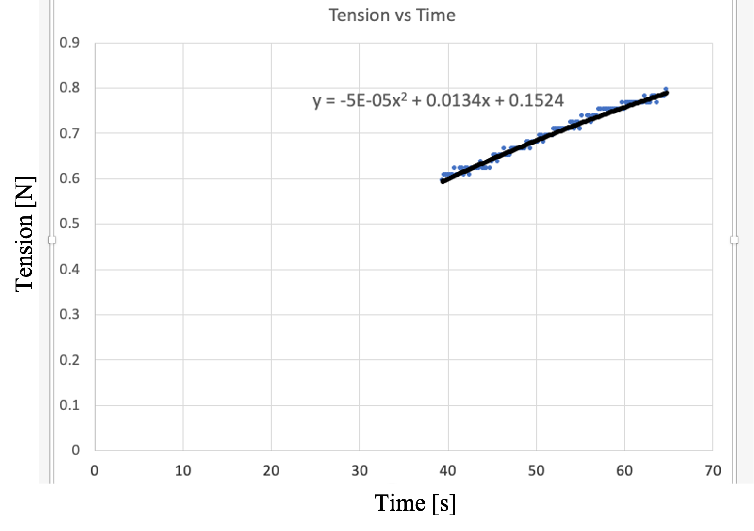
\[ T(t) = -\alpha t^2 + \beta t + \gamma; \qquad t_1 \leq t < t_2. \]
Where \(\alpha,~\beta,\) and \(\gamma\) are constants given by:
\[ \begin{align} \alpha &= \frac{1}{4}\rho A_0 g \kappa_2^2\\ \beta &= \rho A_0 g \kappa_2 \sqrt{y_0 + h_0} + \frac{1}{2}\rho A_0 g \kappa_2^2 t_1\\ \gamma &= mg - \rho A_0 h_0 g - \rho A_0 g \kappa_2 \sqrt{y_0 + h_0} t_1 - \frac{1}{4}\rho A_0 g \kappa_2^2 t_1^2 \end{align}\]
Therefore the magnitude of the tension can be written as:
\[ \begin{align} T(t) = \left\{ \begin{array}{cc} mg - \rho A_0 h_0 g \quad; & \hspace{5mm} 0 \leq t < t_1 \\ -\alpha t^2 +\beta t + \gamma \quad; & \hspace{5mm} t_1 \leq t < t_2 \\ mg \quad\qquad\qquad; & \hspace{5mm} t_2 \leq t < t_3\\ \end{array} \label{eq:Tfull} \right. \end{align} \]
Taking the derivative of the tension with respect to time we get:
\[ \begin{align} \frac{dT}{dt} = \left\{ \begin{array}{lc} 0 \qquad; & \hspace{5mm} 0 \leq t < t_1 \\ -2\alpha t +\beta \quad; & \hspace{5mm} t_1 \leq t < t_2 \\ 0 \qquad; & \hspace{5mm} t_2 \leq t < t_3\\ \end{array} \label{eq:dTdtfull_compact} \right. \end{align} \]
Substituting the second equation of Eq. \eqref{eq:dTdtfull_compact} into Eq. \eqref{eq:v1fromdTdt} we get \(v_1(t)\) as:
\[ \boxed{v_1(t) = \frac{-2\alpha t +\beta}{\rho A_0 g} \qquad;\quad t_1 \leq t < t_2} \label{eq:v1final} \] and we can immediately determine \(v_2(t)\) as:
\[ \boxed{v_2(t) = \frac{(A_1-A_0)(\beta-2\alpha t)}{\rho A_2 A_0 g} \label{eq:v2final} \qquad;\quad t_1 \leq t < t_2.}\]
If you would like to learn more about Bernoulli's Equation, see the following video.