Circular Motion Lab

Objectives

  • Study the relationship between tangential velocity (\(v\)) and angular velocity (\(\omega\)) in circular motion.
  • Study the relationship between centripetal acceleration (\(a_c\)) and angular velocity (\(\omega\)) in circular motion.
  • Study the relationship between tangential acceleration (\(a_\textrm{tan}\)) and angular acceleration (\(\alpha\)) in circular motion.

Physics Overview

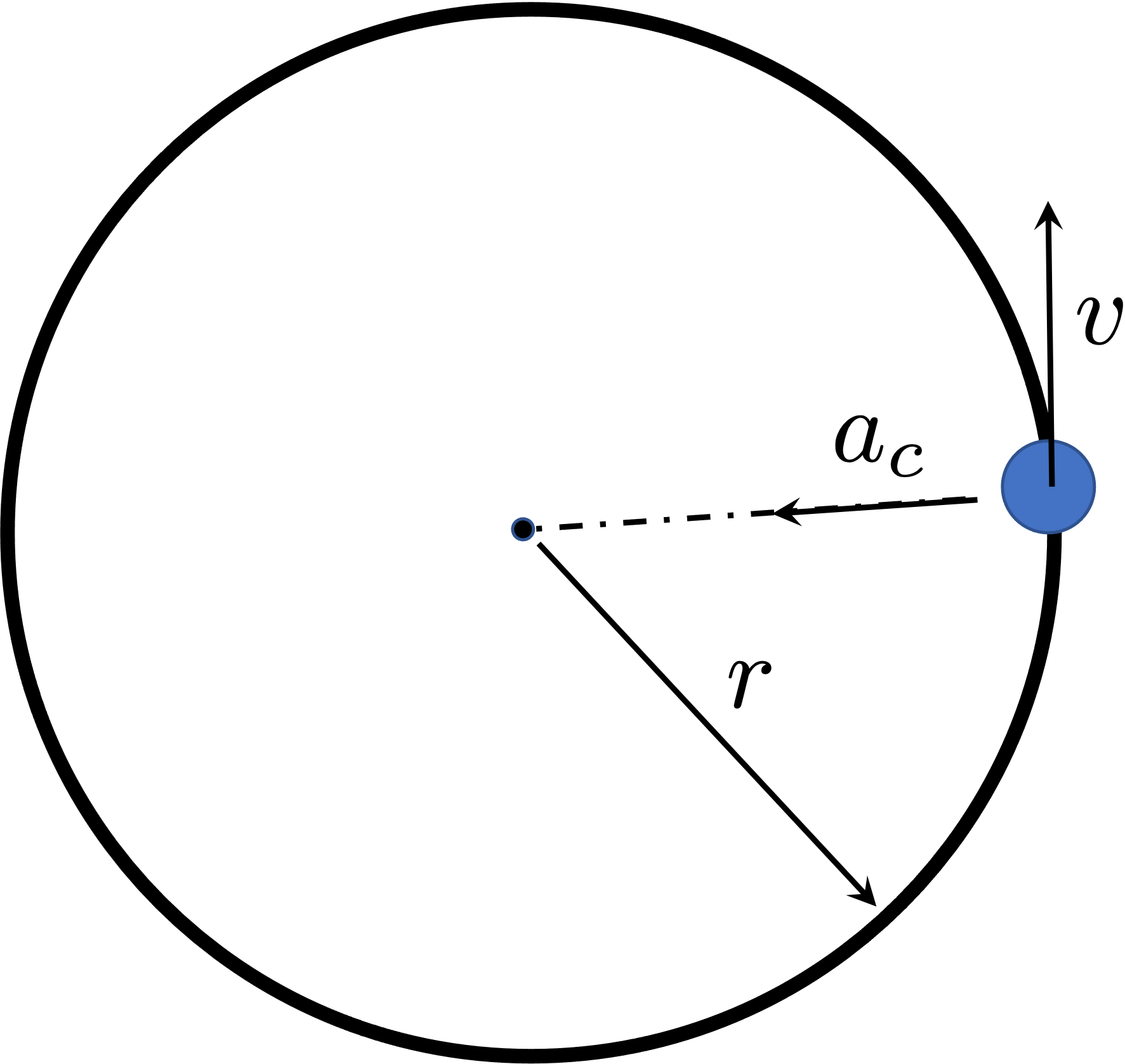
If an object is constrained to move along a circular path, there must be a constraining agency that makes the object move along a circular path. This can be envisioned using the example shown in Figure 1, which shows an object moving along a circle or radius \(r\). At the moment shown, the object has a tangential velocity \(v\), and it has an acceleration that points to the centre of the circle - the centripetal acceleration \(a_c\). This constraining agency is a net force that acts on the object. In general, this force will have two components; a radial and a tangential one. If the tangential component of the force is zero then the motion is uniform circular motion, and if this component is non-zero, then the motion is called non-uniform circular motion.

an object moving along a cirlce

Fig. 1: A small mass \(m\) moves along a circle of radius \(r\). The instantaneous tangential velocity is \(v\) and the centripetal acceleration is \(a_c\).

The rotational velocity or angular velocity of the object as it goes around the circle is defined quite simply as the rate of change of angle with respect to time. Hence it is defined as:


\[ \omega = \frac{d\theta}{dt}, \label{eq:omega_def}\]


and this in turn has a straight-forward relationship with the tangential velcoity;


\[ v = \omega r. \label{eq:vomegar}\]


Thus for an object moving along a circle of a given radius, if the velocity is constant then it implies that the rotational velocity will likewise also be constant. This is the condition for uniform circular motion. In such a scenario the there is no tangential acceleration and the only acceleration that the object has is due to the centripetal force alone, and the centripetal acceleration is given by,


\[ a_c = \frac{v^2}{r} = r \omega^2.\label{eq:a_c}\]


Note that the direction of the centripetal acceleration is perpendicular to the tangential velocity, and therefore it does not change the magnitute of the velocity. However, if there is a tangential acceleration as well, then it has the effect of changing the magnitude of the tangential velocity. Tangential acceleration is defined as,


\[ a_\textrm{tan} = \frac{dv}{dt} = r \frac{d\omega}{dt}.\label{eq:a_tan}\]


The rate of change of the angular velocity (\(\omega\)) with respect to time is by definition the angular acceleration (\(\alpha\)), thus we can write:


\[ a_\textrm{tan} = r \alpha. \label{eq:atan2} \]


Thus when the angular acceleration is zero, then the tangential acceleration is zero and the object executes uniform circular motion, and if it is non-zero then the object executes non-uniform circular motion.


In today's lab you will be experimentally verifying the relationships given in Eqs. \eqref{eq:vomegar}, \eqref{eq:a_c} and \eqref{eq:atan2}.


If you would like to get a quick video refresher about non-uniform circular motion, see the following video.


Apparatus

For carrying out the experiment you will need the following equipment:

  • iOLab Device and corresponding USB Dongle.
  • A computer with iOLab data logging software installed.
  • iOLab accesory kit.
  • Phy 200 iOLab kit.
  • Some string (and scissors).

Give it a go!

give it a go

Procedure

What you will be doing in the experiment is essentially shown in the video below:


This is the procedure to be followed:

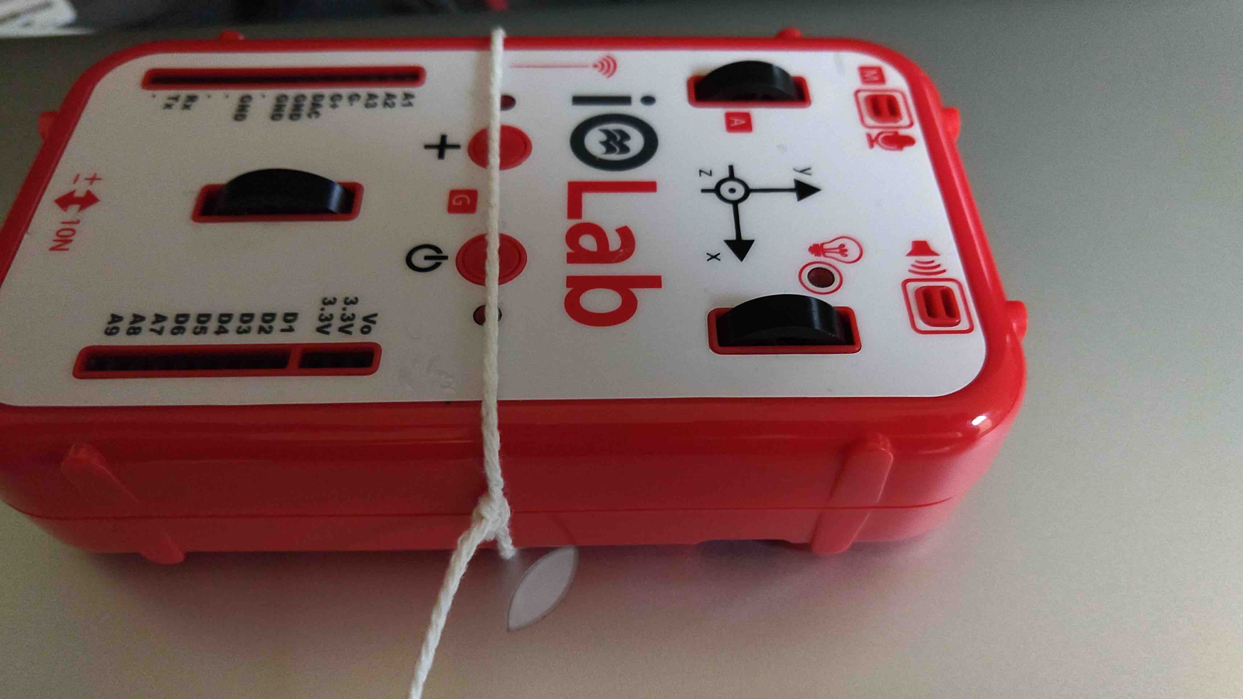
  1. Attach a piece of string to the iOLab device as shown in Figure 2. After tying the string, ensure that the loose end is at least \(18-20~\)cm long as shown in Figure 3.
  2. Measure the length of the loose end of the string and note it down. Add to this half the width of the iOLab device to obtain a measurement of the radius of the circular path that the iOLab device will take.
  3. Turn on the device and and open the data collection software on your computer after plugging in the USB dongle. On the software select the accelerometer, the gyroscope and the wheel sensor. On the wheel sensor we will only require velocity data, so you should deselect wheel position and wheel acceleration.
  4. Place the iOLab device on the table, wheels down, and press record and collect data for approximately \(5\)s.
  5. Place a finger on the loose end of the string and hold it down firmly and while the data is still getting recorded, give the device as push as shown in the video above. Try to push the device along the positive \(y-\)direction. The device should move along a circular path and then come to a stop.
  6. Stop recording the data after the device has come to a full stop.
  7. Export the data to csv files. You should have three csv files in your local directory, one for the acceleration, one for the rotational velocity and the third for the wheel position.

tying a string to the iOLab device

Fig. 2: Tie a string to the iOLab device.

measure the string length

Fig. 3: Measure the length of the loose end of the string.

Data Analysis


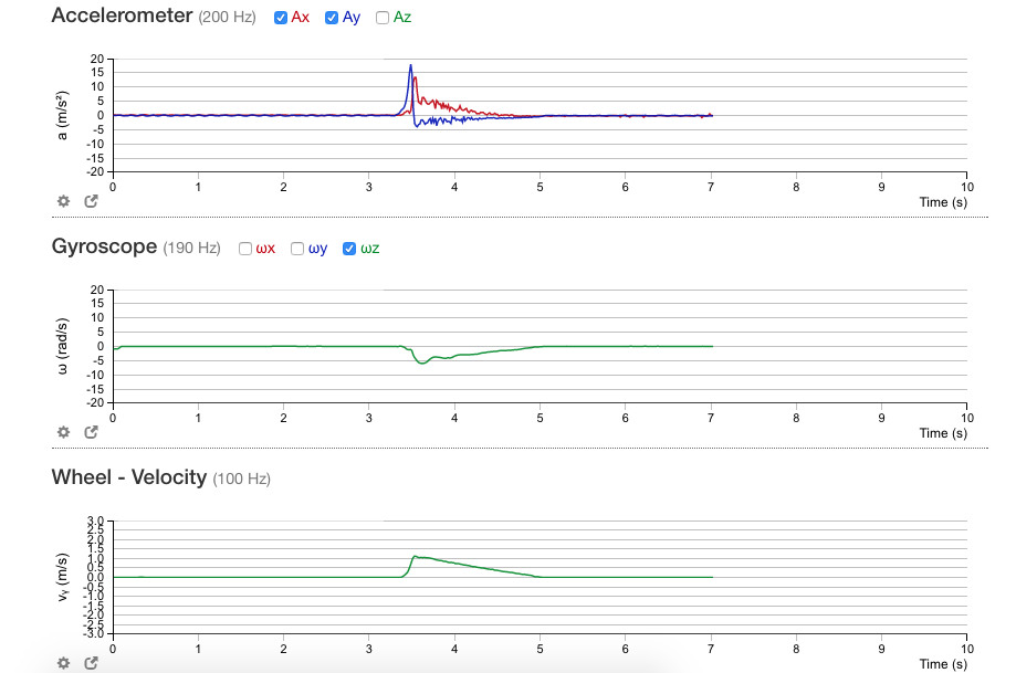
After collecting the data you should have three graphs, one of acceleration vs time, another of the rotational velocity (\(\omega\)) vs time, and a third one showing the wheel velocity in the \(y-\)direction as a function of time. You data should look similar to that shown in Figure 4.


screenshot of acceleration, rotational velocity, and wheel velocity as functions of time.

Fig. 4: Screenshot showing an example of the data collected; acceleration, rotational velocity, and wheel velocity as functions of time. Notice that you only need acceleration in the \(x-\) and \(y-\)directions i.e., \(A_x\) and \(A_y\). Similarly you only need rotational velocity in the \(z-\)direction; \(\omega_z\).

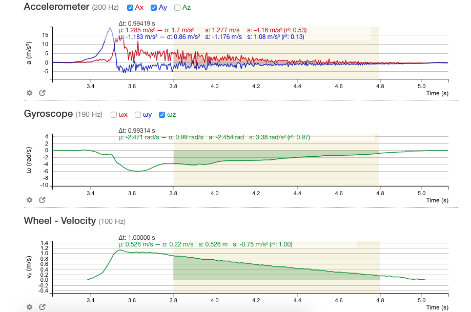
Zoom in on the plots as shown in Figure 5. If you look at the wheel velocity as a function of time, you will notice that the wheel decelerates at a more-or-less constant value - the decline in the velocity is linear. The iOLab device slows down gradually and comes to a stop as seen in the video above. In the exported csv files select a portion of the data from each file when the iOLab device gradually slows down - see for example the highlighted portion in Figure 5.


zoomed in on a portion of the data

Fig. 5: Zoom in on a portion of the data - select a duration of time when the wheel velocity declines at a more-or-less constant rate. In this example, the duration of time selected is approximately \(1~\)s long. Note the beginning and end points of this time interval, then select only that portion of the data from the three exported csv files.

The following video shows how to select the data from the csv files:


Once you have extracted the data as shown in the video above be sure to save the data in a file.


The following video shows you how to analyse the data to confirm that the tangential velocity (\(v\)) is linearly proportional to the rotational velocity (\(\omega\)) and that the centripetal acceleration (\(a_c\)) is proportional to (\(\omega^2\)), and in each case, the constant of proportionality is \(r\); the radius of the circular path.


The video above will allow you to arrive at an experimentally inferred value for the radius of the circular path that the iOLab device moves along. Note this down. How does this compare with the radius of the circular path that you measured earlier, prior to giving the device a push? Once you have completed this analysis, you should be able to verify, within experimental error, Eqs. \eqref{eq:vomegar} and \eqref{eq:a_c}.


Finally, using the analysis tool on the iOLab data collection software, highlight the portion of the data that you exported; refer to Figure 5 above. Note down the slopes of the wheel velocity and the angular velocity; the slopes are the tangential acceleration (\(a_\textrm{tan}\)) and angular acceleration (\(\alpha\)), respectively. Divide the magnitude of the former by the magnitude of the latter and you should have another estimate for the radius (\(r\)) of the cicular path; see Eq. \eqref{eq:atan2} above. How does this compare with the two values you obtained earlier?


Report Considerations

Make sure you include the following in your lab report:

  • A short description of the data analysis you carried out.
  • A plot of \(v\) vs \(\omega\), including the fit (see video above).
  • A plot of \(a_c\) vs \(\omega^2\), including the fit and trendline (see video above).
  • Describe the errors in your measurements.
  • A snapshot of your analysis of the slopes of the velocity and angular velocites (see Figure 5 above).
Questions to answer in the discussion section.
  • How do the two experimentally determined values for \(r\) compare with the measured one?
  • Why do you think the iOLab device slows down to a stop? What is the agency that causes it to decelerate?
  • If you plotted \(a_c\) vs \(\omega\) instead, what would you expect for the relationship between the two? What kind of trendline would be appropriate?