Projectile Motion Lab

Physics Overview

Projectile motion in 2D is simultaneous motion in the x- and y-directions. The two motions are coupled via the time variable "t". When a projectile moves only under the influence of gravity, then it undergoes accerelation only in the y-direction, while the acceleration in the x-direction is zero; i.e., it is linear kinematics in 2D, with the acceleration in the y-direction being equal to that due to gravity (a constant), while the acceleration in the x-direction is zero.

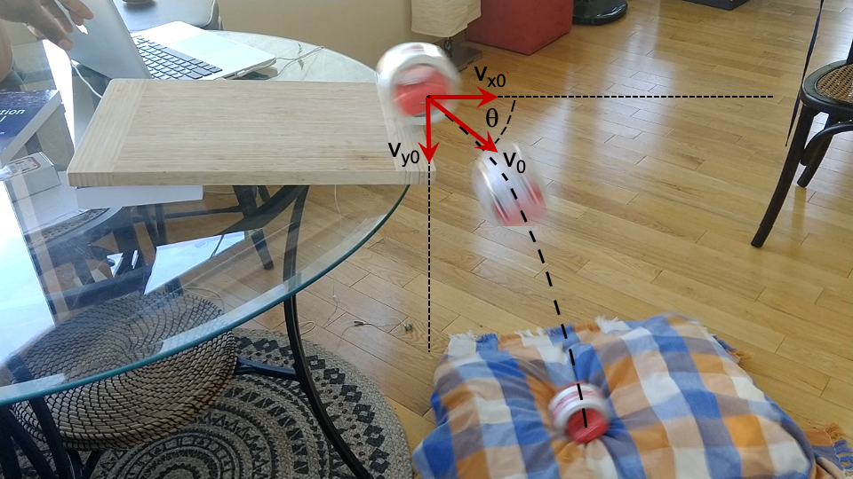
We understand from linear kinematics that if the acceleration is constant then we can write the familiar equations for kinematics. Let us imagine a projectile that is launched into the air at some initial launch velocity of v₀, directed at an angle θ₀ as shown in the figure below.

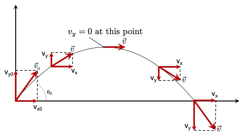
The initial launch velocity v₀ has components in the x- and y-directions of v_x0 and v_y0, respectively. These are given by,

Notice that as the projectile moves through the air, in the y-direction the speed of the projectile changes under the influence of gravity - identically to an object thrown vertically ; the projectile's speed slows down to zero, at which point the projectile has reached the apex of its trajectory - notice that the y-component of the velocity diminishes to zero during the first half of the motion from the launch point up to the apex. Subsequently, the y-component of its velocity then increases and the direction in which the y-component points gets reversed.

On the other hand, the x-component of the velocity is unchanged and remains constant, as there is no acceleration in the x-direction, as a result the x-component can be seen to be constant in Fig. 1.

We can therefore write three equations for kinematics for the motion in each of the two cardinal directions; x and y. This is shown in Table 1.

We can therefore write three equations for kinematics for the motion in each of the two cardinal directions; x and y. This is shown in Table 1.

Notice that in the horizontal direction, i.e., the x-direction, the projectile travels a distance v_x0t in time interval "t". And, in that same time interval it travels a vertical distance given by v_y0t + ½gt², where we have substituted a_y=g.

If you would like to further review projectile motion, then please watch the video below.

Also try experimenting with the PHET simulation below to get an idea of how projectile motion depends on launch angle and launch velocity; in particular pay special attention to the vectors. Note that you can also make the simulation run in full-screen mode by selecting the full-screen option in the options menu (three dots in the lower right corner).

Rolling without slipping

For an object that rolls on a surface without slipping (such as the duct tape roll in this experiment) there is a special relationship between the translational velocity of the object and the rotational (or angular) velocity with which the object rotates about its centre of mass. You will encounter rotational velocity later in Chapter 5, and much later in Chapter 11 you will encounter the concepts of centre of mass and rotational dynamics. Presently suffice it to say that the rotaional velocity, measured about an axis through its centre of mass is related to the translational or linear velocity of the centre of mass via a linear relationship:

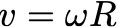
In this experiment you will be measuring ω using the iOLab device and the radius of the duct tape roll is simple to measure. Thus you will be able to determine the translational or linear velocity of the duct tape roll.

Give it a go!

Procedure

The following video shows what you will be doing in the lab - allowing the duct tape with the iOLab device housed inside it to roll down an inclined plane and land on the sponge/cushion on the floor below. While the iOLab is in the air it follows projctile motion. You will use a track in the lab, rather than a cutting board as the incline along which to roll the device.

The procedure to be followed for doing the experiment is given below:

Part - I (incline set up):

1. Set up the track at an incline using the ring stand and the track rod clamp. Attach an angle indicator or use a protractor to measure the inclination. Record the inclination angle (\(\theta\)).
2. Place the yellow sponge on the floor - try to estimate the region where you expect the duct tape roll to land - refer to the video above.
3. Measure and record the vertical drop height from the edge of the track down to the surface of the floor below .
4. Measure and record the outer diameter of the duct tape roll to determine its radius (R).

Part - II (rolling the duct tape and iOLab device):

The following video shows how you will be collecting the data for the experiment.

Here is the procedure to be followed:

1. Gently slide the iOLab device into the duct tape roll as shown in Fig. 1. Make sure that it sits snugly.
2. Plug the dongle into the computer and turn on the device.
3. Turn on the iOLab software and select the gyroscope sensor; a graph showing rotational velocity, \(\omega\) vs time should appear. Leave all three rotational velocities checked, i.e., record all three \(\omega_x\), \(\omega_y\) and \(\omega_z\).
4. Align the lower edge of the track with the edge of the table.
5. Place the duct tape roll with the iOLab device housed inside it in one of the four starting positions on the incline/track (see Fig. 2).
6. Record data for about 5-7 s before letting go of the roll and allowing it to roll down the inclined plane.
7. Stop recording data after the roll has come to a stop on the sponge/floor below.
8. Measure the horizontal distance travelled by the projectile, measured with respect to a point directly vertically below the edge of the incline.
9. Repeat the experiment, i.e., repeat steps 1-8, for the other three starting positions (see Fig. 2); carefully recording and saving the runs each time. When you change the starting position you will change the launch velocity of the projectile.
10. Now change the angle of the incline by a small amount and repeat steps 1-9 above. This will give you data for how the projectile motion depends on the angle of launch.

Report Considerations

Make sure you include the following in your lab report:

• Include snapshots of the raw data graphs of each of your runs (8 in total).
• Include ONE (1) example snapshot showing your analysis of the data (see Fig. 5 above).
• Provide clear plots for:
  1. the horizontal distance travelled by the projectile vs linear velocity (\(v=\omega R\)) at launch; one graph for each angle of inclination.
  2. the time of flight of the projectile vs the linear velocity at launch; one graph for each angle of inclination.
• Discuss the errors in your measurements.
• Describe what you learned from each of the graphs.

Questions to answer in the discussion section.

Refer to Fig. 6 when attempting to answer the questions below.

• How will you confirm the linear relationship between rotational velocity at launch (\(\omega_y\)) and the linear velocity (v) at launch? In other words does your data demonstrate a linear relationship between the two?
• Can you demonstrate this with a plot using your data? If so, show the plot.
• How does the launch angle affect the time of flight and horizontal distance travelled?.
• Does your data for the horizontal distance travelled and the data for the time of flight agree or disagree with theoretical expectations? Explain.

The figure below shows the trajectory of the duct tape as it falls through the air. Notice that at the moment of launch, the velocity vector makes a negative angle with the horizontal. This angle is drawn exaggerated for ease of viewing.